This is a new announcement banner that can be turned on and off

Building a debt amortization schedule in Excel is one of the simplest ways to track how a loan balance changes over time. Whether you’re modeling a term loan, checking repayment assumptions, or monitoring outstanding exposure, Excel’s built-in financial functions make it possible to calculate every payment without building the math from scratch. In this guide, you’ll learn how to build a debt amortization schedule in Excel, calculate principal and interest payments using PMT, PPMT, and IPMT, and understand when a manual spreadsheet becomes difficult to manage.
A debt amortization schedule is a table that breaks down every payment on a loan into two parts: the portion that goes toward interest, and the portion that reduces the principal balance. It also tracks the remaining balance after each payment, all the way through to the final payment at maturity, when the balance reaches zero.
Amortization is a general finance term for spreading a cost, in this case a debt, over a set period through regular payments. A debt amortization schedule is simply the detailed, period-by-period record of that process.
Most amortizing loans, such as term loans, mortgages, and auto loans, follow the same basic pattern: payments are typically fixed in amount, but the mix inside each payment shifts over time. Early payments are weighted more heavily toward interest because the outstanding balance is largest early on. As the balance shrinks, less of each payment goes to interest and more goes to principal, even though the total payment stays the same.
This structure matters beyond simple bookkeeping. Lenders, borrowers, and portfolio teams use amortization schedules to forecast cash flow, calculate outstanding exposure at any point in time, and confirm that payments are being applied correctly.
Before building anything in Excel, it helps to understand the calculation by hand, since every formula in the spreadsheet is just an automated version of these same steps.
To calculate a debt amortization schedule, you need four inputs:
From there, the calculation for each period follows three steps:
Repeat this process for every period until the balance reaches zero. For a loan with a long term, doing this by hand for every payment is impractical, which is why Excel formulas exist to automate each step.
Excel does not have a single built-in “amortization schedule” function, but it has three financial functions that together do all the work.
PMT calculates the total fixed payment for each period, combining both principal and interest.
PPMT calculates the principal portion of a specific payment.
IPMT calculates the interest portion of that same specific payment.
PPMT and IPMT use the same arguments as PMT, but add per to isolate a single period. In a completed schedule, PPMT plus IPMT for any given row should always equal the PMT value for that row. If payments are made at the beginning rather than the end of each period, include the optional type argument in the PMT, PPMT and IPMT functions.
Excel also includes CUMIPMT, which calculates cumulative interest over a range of payment periods.
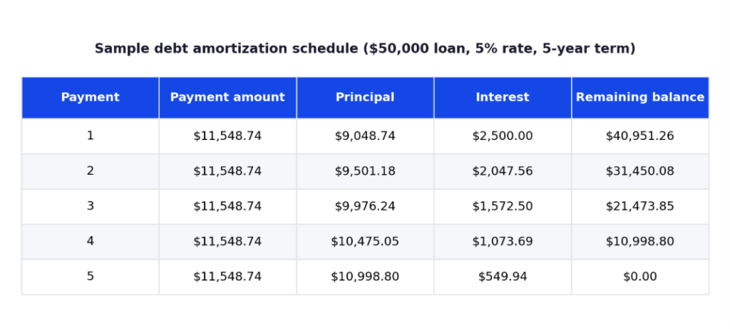
A basic template needs six columns: payment number, payment date, total payment, principal, interest, and remaining balance. The image below shows what a completed schedule looks like for a simple $50,000 loan at a 5% annual rate over a 5-year term with annual payments.

Notice how the principal portion of each payment grows every year while the interest portion shrinks, even though the total payment stays flat. This is the core pattern of every amortizing loan, regardless of size or term.
A reusable template should keep the four core inputs (loan amount, rate, term, frequency) in separate, clearly labeled cells at the top of the sheet, rather than typed directly into formulas. That way, updating the loan amount or rate for a new deal only requires changing one cell rather than rewriting every row.
Follow these steps to build a working schedule from scratch.
A common mistake at this stage is hardcoding the interest rate or loan amount into individual formulas instead of referencing the input cells. This makes the schedule brittle: changing the rate later means editing every row instead of one cell.
Making an extra, or additional, principal payment reduces the outstanding balance immediately, which lowers the interest charged in every subsequent period. Over the life of the loan, this can meaningfully shorten the term and reduce total interest paid, even from a single extra payment made early on.
The mechanics of adding this to an Excel schedule: create an additional column for extra principal payments, then adjust the closing balance formula for that period to subtract both the scheduled principal and the extra payment. From that row forward, every remaining period needs to be recalculated against the new, lower balance.
This is manageable for a one-time adjustment on a single loan. It becomes considerably harder to manage cleanly when:
Each of these scenarios means going back through every affected row and confirming the formulas still reference the correct prior balance. In a single spreadsheet, this is tedious but doable. Across a portfolio of loans or facilities, it becomes a real operational risk, since there is no built-in way for Excel to flag that an old schedule no longer reflects the current terms.
Termgrid is a purpose-built deal management and portfolio monitoring platform for private capital markets. Its amortization feature gives teams a dedicated place to maintain a facility’s amortization schedule, rather than rebuilding one in Excel every time a term changes.
For firms managing amortization across more than a handful of facilities, that is the practical difference: rebuilding a schedule by hand every time something changes, versus keeping one in a system built to hold it.
See how Termgrid’s Amortization tracker works or request a demo to walk through it with a member of the team.
They describe the same thing. “Loan” refers to the specific type of debt instrument, while “debt” is the broader term that also covers instruments like bonds and credit facilities. The underlying calculation, splitting each payment into principal and interest, is identical regardless of which term is used.
Yes, but it requires more manual work. Instead of a single rate applied across the whole schedule, each period’s IPMT and PPMT calculations need to reference that period’s specific rate. This is manageable for a handful of rate changes but becomes harder to maintain accurately as changes become more frequent.
Add a running total column that sums the interest portion of every payment, or use the CUMIPMT function, which calculates cumulative interest paid between two specified periods in a single formula.
Yes, but you’d manually calculate interest and principal every period. PMT automates the payment calculation and is generally the easier approach.
Yes. An extra principal payment reduces the outstanding balance immediately, which lowers the interest charged on every subsequent payment and can shorten the loan’s remaining term. Every row after the extra payment needs to be recalculated against the new balance.
This is usually caused by a mismatch between the nper value used in PMT and the number of periods actually built into the schedule, or a rounding difference from carrying too few decimal places in the payment calculation. Check that the periodic rate, number of payments, and loan amount are consistent across all three functions before troubleshooting further.
Run deals faster. Track covenants in real time. Strengthen portfolio oversight.
Stay in touch with all of our latest updates and articles.